ABSTRACT

This technical report discusses the evaluation of computer-based electrostatic precipitator performance (ESP) models to estimate particulate emissions from coal-fired utility boilers. A field evaluation of the technology was conducted under the Electric Power Research Institute (EPRI) Compliance Assurance Monitoring (CAM) Protocol Development project. The CAM regulation requires that sources provide a demonstration of a "reasonable assurance of compliance" with particulate emission limits. It was believed, and this project has shown, that the use of an ESP performance model is a viable method of providing that demonstration. In addition, and at the request of a number of utilities, continuous particulate matter (PM) monitors were evaluated as a part of this project. The results of the PM monitor evaluation is discussed in another technical paper presented at this conference.

The field test program, which was conducted at Georgia Power Company's Plant Yates, was designed to provide data that can be used in a rigorous evaluation of both the ESP performance models and continuous PM monitors. The test plan was to evaluate three different ESP powering conditions, which would result in three different particulate mass emission levels, each of the 3 weeks of the test program. The first two weeks of testing were conducted back-to-back and the third week of testing was approximately 3 months later. The fundamental premise of this field evaluation was to use the initial week of testing to calibrate the PM modeling/measurement technologies. The second week of testing, conducted immediately following the initial week, would provide information regarding the short-term accuracy and stability of the calibrations. The third week of testing, conducted approximately 3 months following the initial weeks, would provide information regarding the long-term accuracy and stability of the calibrations. This report presents the results of the 3-week field-testing program.

It can be concluded from this project that all of the ESP models evaluated are viable candidates for use under the CAM regulation. The calibrations were stable and the emission predictions were very accurate even after 3 months.

TEST PROGRAM DESCRIPTION

The field test program, which was conducted at Georgia Power Company's Plant Yates, was designed to provide data that can be used in a rigorous evaluation of both the ESP performance models and continuous PM monitors. The test plan was to evaluate three different ESP powering conditions, which would result in three different particulate mass emission levels, each of the 3 weeks, for a total of nine independent test conditions. The first two weeks of testing were done back-to-back and the third week of testing was approximately 3 months later. The fundamental premise of this field evaluation was to use the initial week of testing to calibrate the PM modeling/measurement technologies. The second week of testing, conducted immediately following the initial week, would provide information regarding the short-term accuracy and stability of the ESP models and instruments calibrations. The third week of testing, conducted approximately 3 months following the initial weeks, would provide information regarding the long-term accuracy and stability of the calibrations.

During the first week three series of tests were performed. The initial tests were conducted with the ESP operating in an "as found" condition. The two other test conditions were obtained by simply deenergizing ESP fields. This simulates the complete loss of ESP sections, which is the most common failure mode of an ESP. During the second week of testing, the higher dust loading conditions were achieved by turning down power on all ESP sections in increments. This mode of ESP operation simulates problems attributable to high resistivity ash or close clearance. Five stack sampling runs were conducted at each of the three test conditions. Each stack sampling run consisted of performing two simultaneous particulate emission tests using EPA Method 17. Simultaneous Method 17 tests were performed for two reasons: (1) to evaluate the variability of the test method when tests are performed with two independent sampling trains and (2) to provide a mechanism for rejecting "invalid" test data. The ESP inlet was also tested for particulate mass loading, particle size distribution and ash resistivity on Monday of each test week.

Description of Test Site

Yates Unit 7 has a conventional Combustion Engineering tangentially-fired boiler with steam conditions of 1000° /1000° F and a rated capacity of 360 MWe. The unit, which began commercial service in 1974, burns eastern bituminous coal and is dispatched as a load-following unit. Low NOX burners with separated overfire air were installed on Unit 7 during a 1994 outage. For purposes of this test program, the load was fixed at 350 MWe. Yates Unit 7 is subject to a particulate emission limit of 0.24 lb/10⁶ Btu. The unit also has a 6-minute average opacity limit of 40 percent, and a 4-hour average opacity limit of 34 percent.

ESP inlet testing was conducted in two rectangular air heater outlet ducts. The test ports are approximately 40 feet upstream of the ESP inlet plenums. The inlet sampling location was under about 1.6 inches H₂O of positive pressure.

Emission (outlet) testing was conducted in the 16-foot diameter stack at an elevation of 305 feet above grade. Since the outlet (stack) sampling location easily satisfies EPA’s Method 1 criteria of 8 diameters downstream and 2 diameters upstream from flow disturbances, only 12 individual sampling points were required. Southern Research Institute, under subcontract to RMB, performed all particulate emission testing.

A layout of the Yates Unit 7 ESP is shown below. This ESP was recently rebuilt in the original casings with 11-inch plate spacing and rigid, spiked discharge electrodes.

The ESP is comprised of 2 side-by-side boxes, each with 10 electrical and mechanical fields in the direction of gas flow. The first two fields are six-feet long and the remaining fields are three-feet long in the direction of gas flow, for a total ESP treatment length of 36 feet. The plates are 30 feet high. The nominal specific collection area (SCA) is 300 square feet of plate area per 1,000 cubic feet of flue gas. The ESP internal velocity of 4.5 ft/sec is fairly low.

Discussion of Test Setup and Results

The initial week of testing at Yates went well; however, a couple of test conditions were encountered that were originally thought to be "unrepresentative." The first test series, with the ESP operating in an "as found" condition resulted in a stack particulate emission rate ~ 0.002 lb/10⁶ Btu and 3% opacity. This particulate emission rate was much lower than anticipated, based on previous compliance tests conducted on this unit. The second test day produced a particulate emission rate of ~ 0.06 lb/10⁶ Btu and 15% opacity. The third test day yielded ~ 0.23 lb/10⁶ Btu and 25% opacity. This represented a desired high dust loading condition, although a significant number of "chunky" carbon particles were observed on the Method 17 filters. While these results were not exactly what were anticipated, the results provide for a better understanding of how the ESP responds and, combined with a understanding of the carbon carryover (rapping reentrainment) problem, facilitated subsequent test settings. In essence, it was not possible to cover the range of emissions needed for the second week by only reducing power in the ESP as originally planned. It was necessary to combine power reduction with removal of sections, to achieve the desired range of results.

Our initial concern with the first week’s tests was that two of the conditions appeared to be unrepresentative of a "typical" ESP. We had extremely low loading on the first day and significant rapping reentrainment the last day. After some thought, we are convinced that the reentrainment condition is probably fairly representative, as will be discussed below.

Week 1 Testing

Previous compliance tests had shown a particulate emission rate of ~0.01 lb/10⁶ Btu. Upon arrival at Plant Yates it was discovered that the ESP had two full (7AD and 7AF) sections and one-half (7AG East) section out on A box and one full section (7BB1) out on B box. The opacity was 3-4%. Therefore, the first ESP outlet test was done expecting about 0.01 to 0.02 lb/10⁶ Btu emission rate - not 0.002 lb/10⁶ Btu. As may be imagined, a rate of 0.002 lb/10⁶ Btu is much lower than most all of the ESPs in the U.S. Also, the very low grain loading can cause problems with the ESP models and may be problematic for the calibrations of some of the PM monitors. Fortunately, the accuracy of the ESP models and the PM monitors is not critical at such low particulate concentrations.

In order to achieve the 0.06 lb/10⁶ Btu tests, 60% (the front four fields on the A box plus the fields already out and the first five fields plus 7BG on the B box) of the ESP was deenergized. The remaining four fields were on automatic voltage control and the opacity was in the range of 12-15%. To get the third condition, only one more field on one box (7AC) was deenergized. The opacity increased 26%.

This last condition was expected to result in a mass loading of about 0.10 lb/10⁶ Btu. Apparently, the point was reached where rapping reentrainment of relatively large unburned carbon particles (i.e., small but large relative to other flyash particles) became a major factor. These large carbon particles were probably in a size range where the opacity monitor is insensitive; therefore, the opacity/mass relationship deteriorates. In other words, the particles contribute a significant amount of mass but little opacity. This is the classical reason why opacity monitors are often not good particulate monitors – when the particle size distribution changes, the opacity/mass relationship changes.

While the last test condition has been previously described as "unrepresentative", it is believed that many units probably have the same high carbon content ash particles because of low NO_x burner conversions combined with short furnaces. It is also interesting to note that the ESP inlet particle size distribution was shifted toward a larger particle size than is usually considered normal for a pulverized coal boiler. A normal mass median diameter is usually about 16 microns and the result from Yates was around 21 microns during the first week of testing.

Week 2 Testing

The test procedure for the second week was the same as for the first week except that instead of taking complete ESP fields out of service, test conditions were established using a combination of overall power reduction and some fields out. In addition, the first test was not done at full ESP power because there did not appear to be any need to test again at the very low emission rate.

ESP inlet mass loading, ash particle size distribution and resistivity tests were performed on Monday and the inlet results were very similar to those from the first week. ESP outlet tests were performed on Tuesday – Thursday.

Week 3 Testing

The test procedure for the third week was virtually a carbon copy of the second week but conducted three months later. Combinations of fields out of service and power reductions were used to obtain the desired particulate loadings. It should be emphasized, however; that no effort was made to duplicate the conditions from the second week. After all, the objective of the project is to evaluate how well the particulate measurement/estimation techniques predict the particulate concentration, no matter what the conditions.

Again, ESP inlet tests were performed on Monday and the inlet mass loading was similar to that from weeks 1 and 2. We did, however note an upward shift in the mass median particle size from 21-24 microns during weeks 1 and 2 to approximately 31 microns during week 3.

RESULTS OF STACK AND ESP INLET TESTING FOR WEEKS 1, 2 AND 3

The results of the particulate emission tests conducted in the stack during all three weeks of testing are summarized in Table 1.
  

The last column of Table 1 presents the percent difference (defined as the difference between a pair of runs divided by the mean of the runs) between each set of paired runs. With the exception of three sets of tests conducted on the very first day of testing (06/03/98), the precision of the paired runs was very good. We expected Run 2 to be biased "high" because of probe contact with one of the sampling ports. However, Run 1 was retained for statistical purposes; retention of Run 1 is justified by its numerical agreement with the other tests conducted on 06/03/98. The fourth and fifth set of tests (Runs 7, 8, 9, and 10) also exhibited a higher percent difference than is desired. However, we do not believe this is problematic because the computed percent difference is mostly dictated by the low mean concentration (i.e., ~ 2 mg/m³).

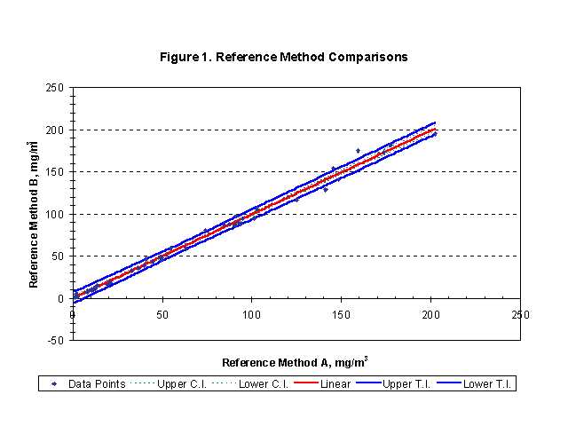
In keeping with our desire to evaluate the contribution of reference method variability to the variability of CAM protocols (whether PM monitors or ESP models), the Method 17 test results were subjected to the identical evaluation that were used for the PM monitors. This evaluation is to apply the proposed EPA PM Monitor Performance Specification (PS) 11 statistics. Figure 1 shows the odd number reference method tests plotted on the x-axis versus the even number tests on the y-axis. The PS 11 linear regression line, confidence intervals and tolerance intervals are also shown.

The confidence intervals are not very useful because all they tell us is that, if the entire experiment was repeated, there is a 95% probability that the new regression line would lie between the confidence intervals. The tolerance intervals are of the most interest because they predict that, if additional data points are taken in the original data set, there is a 95% probability that 75% of the new data points will fall between the tolerance intervals.

The width of the tolerance interval in Figure 1, in the y-direction, is approximately 12 mg/m³ and that width is driven by the maximum observed error (in mg/m³), or the error at the highest test point. This is good because the compliance point is exactly where we are interested in the accuracy of the reference test, PM monitors or ESP models. It should be noted that for CAM purposes owner/operators are only likely to be concerned with the upper tolerance interval or the potential overestimate. (However, EPA is most likely to be concerned with the potential underestimate.) In the case of the Method 17 tests, the width of the upper tolerance interval as well as the lower tolerance interval is about 6 mg/m³, which at a particulate concentration of 75 mg/m³ is 8 percent.

Table 2 shows the result of the ESP inlet testing. 
 

The average particle size mass median diameter (MMD) for Weeks 1 and 2 are similar and probably within experimental error. As can be seen in Table 2, during Week 3 there was an obvious shift in the ESP inlet particle size. The reason for this shift is unknown (pulverizer wear is suspected) but is believed to be fortuitous with respect to the objectives of the test program. Particulate mass and opacity monitors are usually sensitive to particle size distribution changes and this presented the opportunity to evaluate that effect both on the particle monitors as well as the ESP performance model. Another fact that should be noted is that all of the particle size distributions have an MMD that is somewhat larger than the 16 micron MMD normally expected on a pulverized coal unit firing an Eastern bituminous coal. In addition, the Sigma (geometric standard deviation) of the particle size distribution was consistent during all three weeks of testing but was considerably narrower (2.5 versus 4.2) than the generally assumed default value.

Ash resistivity measurements were also done on the ESP inlet. The resistivity was fairly consistent for all three weeks of testing and ranged from 1.1 x 10¹¹ to 5.8 x 10¹¹ ohm· cm and averaged 3.7 x 10¹¹ ohm· cm. Ash resistivity measurements were difficult to make because of the relatively high carbon content of the ash. It was obvious; however, that there were no resistivity problems because of the very high current being carried in many of the ESP sections.

ESP MODEL DISCUSSION

A primary objective of this project was to evaluate the use of ESP performance models as tools for demonstrating a reasonable assurance of compliance under the CAM rule. To provide a complete evaluation of the publicly available models, the EPRI ESPM, SoRI and EPA ESPVI performance models were evaluated. The EPRI model is available to EPRI members and the SoRI and EPA models are in the public domain and can be obtained by anyone.

In evaluating the models, we treated them even more rigorously than the particulate monitors. Each model was "calibrated" to one central test from the first week of testing using the available model fitting adjustments (discussed later). These fitting adjustments were then fixed for all other model runs both during the first week and the two subsequent weeks of testing. The only changes that were made to the model from run to run was to set up the correct number of ESP fields in service and to enter the actual voltages and currents.

Model Setup

Our experience has been that the secondary voltage meters on ESPs are usually out of calibration. Since we had access to precision voltage dividers, calibration curves were developed for all the in-service meters. This was done because the ESP models are fairly sensitive to ESP voltage levels.

Basic model input data sets were then prepared for each tested configuration. These input data sets generally represented the number of fields in-service on the ESP and the specific voltages and currents in each field during each test. The models were then run to evaluate the results. In most cases it was necessary to run a model for the A side of the ESP and a separate model for the B side because the number of fields in-service and the voltages and currents were different. The results of the two models were then averaged.

As discussed previously, the ESP inlet particle size distribution had a mass median diameter (MMD) that was somewhat larger than the default value in the model (21-30 versus 16). We also found that the geometric standard deviation of the particle size distribution was consistent during all three weeks of testing but was considerably narrower than the default (2.5 versus 4.2) used by the models. These were very important findings because none of the models would have worked very well with the default values. Considering our recent experience with the models, we are becoming more convinced that low NO_X burner conversions and the shift to Western coal have made the present model default values out of date. More information on the ESP inlet particle size distribution resulting from present day operation needs to be developed so that new default values can be developed. It may also be possible to obtain a representative particle size distribution and standard deviation by exercising the model in an iterative process. Additional data are likely to be required to prove that such a process will work properly. At the present time, we would definitely have to recommend inlet particle sizing for anyone using an ESP model.

ESP inlet particle size distribution measurements are difficult to make and should only be done by qualified personnel using appropriate equipment, procedures and data reduction techniques. It is essential that the procedures and equipment be as described in "Procedures Manual for the Recommended ARB Particle Size Distribution Method (Cascade Impactors)," California Air Resources Board Report, ARB Contract A3-092-32, Southern Research Institute - Contractor, May 1986

EPRI ESPM Model Results

The basic input data sets containing the test specific ESP voltage and current were then run in the ESPM model and the model "fitting factors" were adjusted to obtain results under several different scenarios. There are several "fitting factors" that can be used in the ESPM model to fit the model to the tested condition. The primary fitting factors are; the velocity sigma, the sneakage fraction and the rapping reentrainment fraction. There are, of course, reasonable ranges for the factors depending on the design of the ESP. Guidance for the ranges is discussed in the ESPM Users Manual and will not be repeated here. Given the design of the Yates 7 ESP, the modeling was started with a velocity sigma of 0.15, a sneakage fraction of 0.10 and a rapping reentrainment fraction of 0.10. As shown in Table 3, this combination gave a fairly good fit for the test points, except the highest, during Weeks 1 and 3 and a reasonable fit for all of Week 2.
  

Since we care more about the accuracy of the model at, or close to, the emission limit of 0.24 lb/10⁶ Btu, it was decided to fit the model to the highest test result and evaluate how this would effect all of the other fits. This was accomplished by simply changing the rapping reentrainment factor from 0.10 to 0.15. (This is a very reasonable adjustment since we observed considerable rapping reentrainment at the two highest emission levels during tests 21-30 and 75-80.) As can be readily seen in Table 3, this produced a perfect fit at the 0.24 lb/10⁶ Btu level and a very good fit at the 0.17 level but the model overestimated at all other test points.

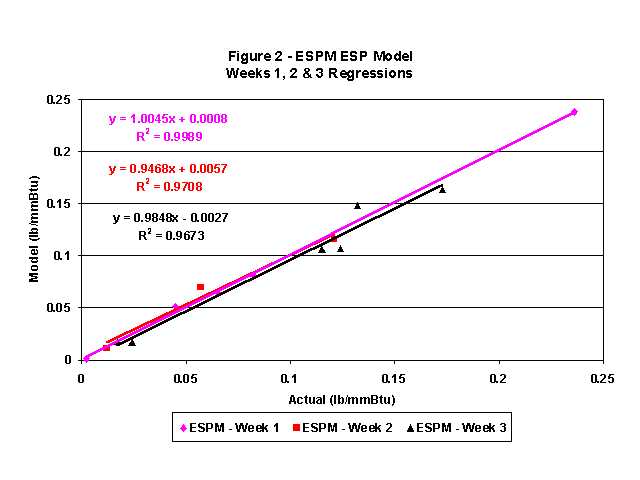
Figure 2 shows the linear regressions for all three weeks of testing using the 0.1 rapping reentrainment factor for all data points except the two highest where 0.15 was used. The equation of the best-fit line for each week along with the correlation coefficient (R²) is also shown. It can be readily seen that the curves are all very similar with slopes of 0.95 to 1.00 and essentially zero intercept (the fits were not forced through zero). In addition, the R² for all of the linear regressions is very high. In other words, the ESPM model does an excellent job of predicting the emissions over an extremely wide operating range of the ESP.

Southern Research Institute Model

The Southern Research Institute (SoRI) ESP performance model was the first ESP computer model developed and was originally designed to run on mainframe computers. It has since been converted to operate on personal computers. It runs very fast (all of the models run in a few seconds on a Pentium based PC) and has the capability of running multiple input data sets in one computer run. It does not, however, have a rapping reentrainment fitting factor like ESPM. The only fitting factors available are a sneakage factor and a velocity sigma factor. We used the sneakage factor to fit the model.

To calibrate the model, an initial matrix of reasonable sneakage factors and velocity sigma factors was set up and the model was run through this matrix to find the best fitting combination. This combination was a sneakage factor of 0.01 and a velocity sigma of 0.10. (Please note that the various models do not necessarily treat factors that have the same name identically with respect to the mathematics of the model.) This combination matched all of the actual data fairly well, except for the two highest data points. To duplicate the past experience with ESPM, another series of runs were made keeping the velocity sigma constant at 0.10 and increasing the sneakage factor incrementally until there was a fit on the first week. This happened at a sneakage factor of 0.17. The model was then run at that set of factors for the high point from the third week. A complete set of model runs was not made with the 0.17 sneakage factor because all would have over predicted the actual emissions. Table 4 shows the results of the SoRI ESP model runs.
  

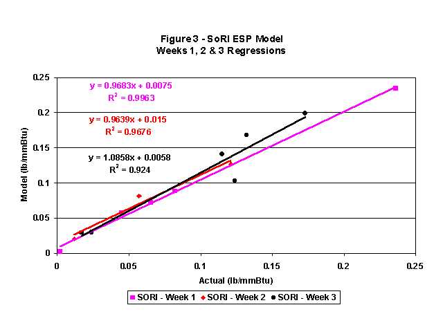
Figure 3 shows the linear regressions for the SoRI model for all three weeks of testing using the 0.01 sneakage factor for all data points except the two highest where 0.17 was used. As with the ESPM graph, the equation of the linear best-fit line for each week along with the R² is also shown. The best-fit statistics for the SoRI model curves are not as good as those for the ESPM model but are still excellent. The slopes vary from 0.96 to 1.09 and the zero intercepts are low. The R² for all of the linear regressions are greater than 0.92. It appears that the SoRI model also provides an excellent prediction of the particulate emissions.

EPA ESPVI 4.0 Model

The EPA ESPVI model is similar to the EPRI ESPM model because the developer/programmer was the same person. By modern standards, the EPA model has a rather old-fashioned, "user hostile" DOS interface, and there are clearly some internal code differences between the two models because the results are slightly different.

In essence, the process for fitting the EPA model followed exactly the same procedure that had been used for the EPRI model. It is interesting to note that the best fit between the model and the field data occurred with almost exactly the same fitting factors as were used for the EPRI ESPM model. These were a velocity sigma of 0.15, a sneakage fraction of 0.10 and a rapping reentrainment fraction of 0.08. Again, the rapping reentrainment fraction had to be raised to 0.14 to get a reasonable fit on the two highest data points. The results from the EPA ESPVI model runs are shown in Table 5.
  

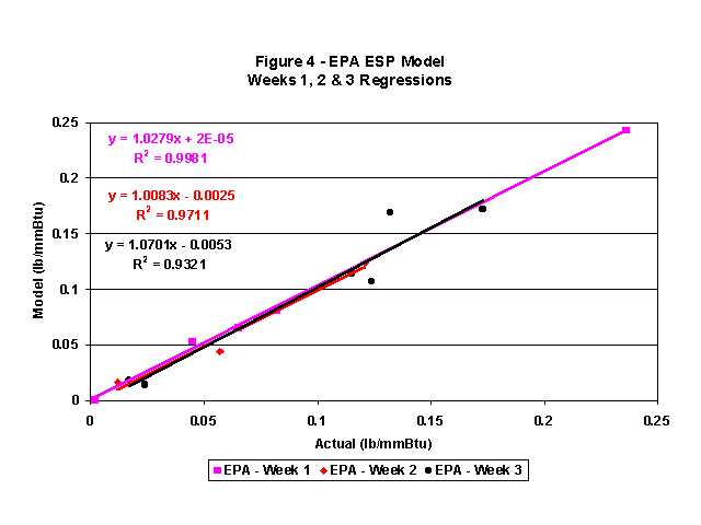
Figure 4 shows the linear regressions for the EPA model for all three weeks of testing using the 0.08 rapping fraction for all data points except the two highest where 0.14 was used. As with the previous graphs, the equation of the linear best-fit line for each week along with the R² is also shown. The best fit statistics for the EPA ESPVI model curves are excellent. At first glance, they appear even better than for the EPRI ESPM model because all of the best-fit lines are stacked closely together. However, upon closer examination it is noted that the range of slopes and R² is higher for the EPA model than for the EPRI model. This is not meant to be a negative comment because the EPA model clearly produces excellent results.

Opacity Evaluation

The primary use for an ESP model under CAM is to predict particulate mass emissions rather than opacity because all major utility boilers have opacity monitors. There are, however, situations like the development of a periodic monitoring procedure or evaluation of ESP upgrades where one would desire confidence in the models’ opacity predictions. Obviously, this project developed the information necessary to evaluate the opacity predictions and the results were quite good.

Table 6 below summarizes the actual opacity from the plant opacity monitor and the opacity predicted by the ESP models. There appears to be approximately a 3% high opacity bias on the plant opacity monitor as shown by the 3.5% opacity reading during Tests 1-10 when the emissions were extraordinarily low. 
 

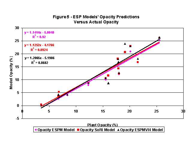
Figure 5 shows a graph of all three models opacity predictions versus the plant opacity monitor readings. All three weeks of data have been lumped together for this comparison. It is interesting to note that all of the linear fits are similar. All also have a negative y-intercept, reflecting the opacity monitor bias.

CONCLUSIONS

1. The paired Method 17 sampling procedure used for these tests shows that very good measurement precision can be achieved across a wide range of power plant particulate emission levels.
2. The total tolerance interval width for the Method 17 measurements, at an assumed emission limitation of 0.1 lb/10⁶ Btu and based on 45 paired runs, was 12 mg/m³.
3. The ESP inlet particle size distribution and geometric standard deviation was somewhat different than has been observed in past tests for Eastern bituminous coals. The ESP inlet particle MMD ranged from 21.5 to 24.4 microns for the first two weeks of testing and was 30.9 during the third week. The typical modeling "default" value is 16 microns. The geometric standard deviation was 2.5 during all three weeks of testing in comparison to the generally accepted range of 3.7 to 4.2. We believe the skewed particle size distribution and geometric standard deviation is due to the retrofit of low NO_X burners in a short furnace. Therefore, the skewed distribution may be a common occurrence on many utility boilers since low NO_X burners have been retrofitted to most coal-fired boilers.
4. The EPRI ESPM and EPA ESPVI ESP performance models gave excellent results when modeling the ESP. The SoRI model also produced acceptable results. After calibration to the first week of data, all three models produced linear regression fits that were very similar for the second and third week of testing. The slope of the linear best-fit lines was very close to 1.0 and most R² values were 0.95 or better. This result is extremely encouraging because it shows that ESP models can be used to demonstrate a reasonable assurance of compliance under the EPA CAM rule.
5. All of the ESP models also predicted opacity very well. This ability can be helpful when using the ESP models to evaluate ESP modifications and upgrades. It will also be useful for designing periodic monitoring approaches.
6. Lastly, it would be very helpful to evaluate the performance of ESP performance models and continuous PM monitors on boilers firing subbituminous coal because the fly ash characteristics are so different from that of bituminous coal.